Induction motor is represented by fifth order nonlinear differential equation as

$$\begin{align*} \dot{i}_{sa} &={MR_{r} \over \sigma L_{s}L_{r}^{2}}\phi_{ra}+{n_{p} M\over \sigma L_{s}L_{r}} \omega\phi_{rb}- \gamma i_{sa}+{1\over \sigma L_{s}}u_{sa} \\ \dot{i}_{sb} &={MR_{r} \over \sigma L_{s}L_{r}^{2}}\phi_{rb}- {n_{p} M \over \sigma L_{s}L_{r}}\omega\phi_{ra}-\gamma i_{sb}+{1\over \sigma L_{s}}u_{sb} \\ \dot{\phi}_{ra} &=-{R_{r}\over L_{r}}\phi_{ra}-n_{p}\omega \phi_{rb}+{MR_{r} \over L_{r}}i_{sa} \\ \dot{\phi}_{rb} &=n_{p}\omega\phi_{ra}-{R_{r}\over L_{r}}\phi_{rb}+{MR_{r}\over L_{r}} i_{sb}\cr \dot{\omega} &={n_{p} M \over JL_{r}}(\phi_{ra}i_{sb}-\phi_{rb}i_{sa})-{fv\over J}\omega-{1\over J}T_{l}, \end{align*}$$

where $i_{sa}, i_{sb}, \phi_{ra},\phi_{rb}$ and $\omega$ denote stator currents, rotor fluxes, and angular velocity, respectively, and $u_{sa}$ and $u_{sb}$ denote stator voltage inputs. The parameters $\sigma$ and $\gamma$ are defined as $\sigma = 1-M^2/L_sL_r, \gamma = (L_r^2r_s+M^2R_r)/\sigma L_s L_r^2 \cdot M, L_s, L_r, R_s$ and $R_r$ denote the mutual inductance, the self-inductances, the resistances, respectively. The subscript $a$ and $b$ denote the components of a vector with respect to a fixed stator reference frame and $s, r$ stand for stator and rotor of motor. $n_p, f_v, J, T_l$ are the number of pole-pair, the co-efficient of viscous damping, the inertia of rotor, and the load torque. We assume that the state variables $i_{sa}, i_{sb}, \omega$ are available for measurement and $T_l$ has a unknown constant value, that is, $\dot{T}_l=0$ . As a result, the model of induction motor can be rewritten into the form

$\eqalignno{ \dot{x}_{i} & =A_{i} (u, y_{i+1}, \cdots,y_{p})x_{i}\cr & +g_{i}(x_{1}, \cdots, x_{i},; u; y_{i+1}, \cdots, y_{p}) \cr & y_{i}=C_{i}x_{i}, 1\leq i \leq p}$

as follows:

$\eqalignno{ & \dot{x}_{1}=\left(\matrix{ 0 & A_{11}(y_{2})\cr 0 & 0}\right)x_{1}+g_{1}(x_{1}, u, y_{2})\cr & \dot{x}_{2}=\left(\matrix{ 0 & A_{21}\cr 0 & 0}\right) x_{2}+g_{2}(x_{1}, x_{2}, u)\cr & y_{1}=C_{1}x_{1}\cr & y_{2}=C_{2}x_{2},}$

where $x_1=[i_{sa},i_{sb},\phi_{ra},\phi_{rb}]^T$, $x_2=[\omega,T_l]^T$, $y_1=[i_{sa},i_{sb}]^T$, $y_2=\omega$, $u=[u_{sa},u_{sb}]^T$ and

$\eqalignno{ & A_{11}= \left(\matrix{ MR_{r}/ \sigma L_{s}L_{r}^{2} & (n_{p}M/\sigma L_{s}L_{r})y_{2}\cr -(n_{p}M/ \sigma L_{s}L_{r})y_{2} & M R_{r}/\sigma L_{s}L_{r}^{2}}\right)\cr & A_{21}=\left(\matrix{ -{1\over J}}\right)\cr & g_{1}=\left(\matrix{ -\gamma i_{sa} +(1/ \sigma L_{s})u_{sa}\cr -\gamma i_{sb} + (1/\sigma L_{s})u_{sb}\cr -(R_{r}/L_{r})\phi_{ra}-n_{p}y_{2}\phi_{rb}+(MR_{r}/L_{r})i_{sa}\cr n_{p}y_{2}\phi_{ra} -(R_{r}/L_{r})\phi_{rb}+(MR_{r}/L_{r})i_{sb}}\right)\cr & g_{2}=\left(\matrix{(n_{p}M/JL_{r})(\phi_{ra}i_{sb})-(\phi_{rb} i_{sa}) - (f_{v}/J)\omega)\cr 0}\right)}$

The hydrostatic transmission dynamics is represented by a nonlinear fourth order state-space model

$$\begin{align*} \dot{q}_{1}(t) &= -a_{11}q_{1}(t)+b_{11}u_{1}(t) \\ \dot{q}_{2}(t) &= -a_{22}q_{2}(t)+b_{22}u_{2}(t) \\ \dot{q}_{3}(t) &= a_{31}q_{1}(t)p(t)-a_{33}q_{3}(t)-a_{34}q_{2}(t)q_{4}(t) \\ \dot{q}_{4}(t) &=a_{43}q_{2}(t)q_{3}(t)-a_{44}q_{4}(t), \end{align*}$$

where $q_1(t)$ is the normalized hydraulic pump angle, $q_2(t)$ is the normalized hydraulic motor angle, $q_3(t)$ is the pressure difference [bar], $q_4(t)$ is the hydraulic motor speed [rad/s], $p(t)$ is the speed of hydraulic pump [rad/s], $u_1(t)$ is the normalized control signal of the hydraulic pump, and $u_2(t)$ is the normalized control signal of the hydraulic motor. It is supposed that the external variable $p(t)$ , as well as the second state variable $q_2(t)$ are measurable. In given working point the model parameters are

$\eqalignno{& a_{11}=7.6923 \qquad a_{22}=4.5455 \quad a_{33}=7.6054.10^{-4} \cr &a_{31}=0.7877 \qquad a_{34}=0.9235\quad\ b_{11}=1.8590.10^{3} \cr &a_{43}=12.1967 \quad\ \ a_{44}=0.4143\quad b_{22}= 1.2879.10{}^{{3}}}$

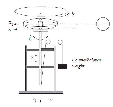
We consider the attached image where the VARIO helicopter mounted on an experimental platform is represented. It is important to say that in this particular case the helicopter is in an OGE condition. The effects of the compressed air in take-off and landing are then neglected. The model has the form

$$M(q)\ddot{q}+C(q,\dot{q})\dot{q}+G(q)=Q(u),$$

where $M(q)\in\mathbb{R}^{3\times3}$ is the inertia matrix, $C(q,\dot{q})\in\mathbb{R}^{3\times3}$ is the Coriolis matrix, $G(q)\in\mathbb{R}^3$ is the vector of conservative forces, $Q(u)=\begin{bmatrix}f_z & \tau_z & \tau_\gamma \end{bmatrix}^{\mathrm T}$ is the vector of generalized forces, $q = \begin{bmatrix} z & \phi & \gamma \end{bmatrix}^{\mathrm T}$ is the vector of generalized coordinates and $u=\begin{bmatrix}h_M & h_T \end{bmatrix}^{\mathrm T}$ is the vector of control inputs. Here $f_Z, \tau_Z$ and $\tau_{\gamma}$ are the vertical forces, the yaw torque and the main rotor torque, respectively. The height $z < 0$ upwards, $\phi$ is the yaw angle and $\gamma$ is the main rotor azimuth angle.

$M(q)=\begin{bmatrix} c_0 & 0 & 0 \\ 0 & c_1 + c_2 \cos^2{(c_3\gamma)} & c_4\\ 0 & c_4 & c_5 \end{bmatrix},$

$C(q,\dot{q})=\begin{bmatrix} 0 & 0 & 0\\ 0 & c_6\sin{(2c_3\gamma)}\dot{\gamma} & c_6\sin{(2c_3\gamma)}\dot{\phi} \\ 0 & -c_6\sin{(2c_3\gamma)}\dot{\phi} & 0\end{bmatrix},$

$G(q)=\begin{bmatrix}c_7 \\ 0 \\ 0 \end{bmatrix},$

where $c_i$'s $i = 0, ..., 7$ are the physical constants given in the table below.

The generalized forces vector is given by

$Q(u)=\begin{bmatrix} c_8\dot{\gamma}^2u_1 + c_9\dot{\gamma} + c_{10} \\ c_{11}\dot{\gamma}^2u_2\\ (c_{12}\dot{\gamma}^2 + c_{13})u_1 + c_{14}\dot{\gamma}^2 + c_{15} \end{bmatrix}$

In 2-DOF helicopter, a coupled 2input-2output system can be achieved due to coupling between the pitch and yaw motor torques. The linear 2-DOF helicopter state-space matrices are

$$\begin{align*} A&=\left[\matrix{ 0 &0 &1 &0\cr 0 &0 &0 &1\cr 0 &0 &-{B_{p}\over J_{eq{\_}p}+m_{heli}{l_{cm}}^{2}} &0\cr 0 &0 &0 &-{B_{y}\over J_{eq{\_}y}+m_{heli}{l_{cm}}^{2}}}\right],\\ B &=\left[ \matrix{ 0 &0\cr 0 &0\cr \dfrac{K_{pp}u_{p}}{J_{eq{\_}p}+m_{heli}{l_{cm}}^{2}} & \dfrac{K_{py}u_{y}}{J_{eq{\_}p}+m_{heli}{l_{cm}}^{2}} \cr \dfrac{K_{yp}u_{p}}{J_{eq{\_}y}+m_{heli}{l_{cm}}^{2}} & \dfrac{K_{yy}u_{y}}{J_{eq{\_}y}+m_{heli}{l_{cm}}^{2}} \cr } \right], \\ C &=\left[\matrix{1 &0 &0 &0\cr 0 &1 &0 &0}\right], D=\left[\matrix{0 &0\cr 0 &0}\right], \end{align*}$$

where $\theta(t)$ is the pitch angle and $\psi(t)$ is the yaw angle. $u_p$ and $u_y$ are the control signals applied to pitch and yaw motors, respectively. The amounts of parameters used in this formula are written in the table below.

This is a more complex model of the system in Point-Mass Satellite Moving in a Plane (1).

$$\begin{align*} \dot{y}_{1} &=x_{1,2}+\psi(y_{2}) \\ \dot{x}_{1,2} &=u_{1} \\ \dot{y}_{2} &=u_{2}. \end{align*}$$